Microservices Benchmarking with DeathStarBench

Why this problem

Most distributed systems coursework ends at "deploy it and check that it works." This one asked for something more demanding: deploy the system, instrument it, put it under load, and then explain what you are looking at. The application was DeathStarBench, a benchmark suite from Cornell that implements a realistic social network using more than 20 microservices communicating over Thrift RPC. The services are deliberately polyglot (C++, Java, Go, Node.js and Python), backed by MongoDB, Redis and Memcached, which makes the deployment closer to a production system than a toy.

We wanted to know how deployment topology affects latency, throughput and resource utilisation. That meant three configurations on GKE: a single node running a single replica, a single node running three replicas, and three nodes running one replica each. Kubernetes autoscaling was available to us, but we fixed the node count on purpose. If the scheduler is free to add capacity mid-experiment, any comparison of load-balancing behaviour across the three setups becomes meaningless.

That was the plan. What the project actually turned into was somewhat different.

What the obvious approach gets wrong

The conventional way to observe a Kubernetes workload is to instrument each service with a Prometheus client library, scrape the /metrics endpoints, visualise in Grafana, and trace requests through Jaeger. All of that assumes you own the application code. DeathStarBench's services do not expose Prometheus-compatible /metrics endpoints at all, so there is simply nothing for a scraper to collect.

Jaeger ships with the repository, but the tracing pipeline does not work as delivered. Header propagation between services is incomplete and the services themselves carry no tracing instrumentation, so Jaeger starts cleanly and then shows an empty UI. The bundled version also disagreed with the rest of the stack, which produced startup failures before tracing was even the issue we were trying to solve.

None of the topology questions were answerable under those conditions. We could run load all day and observe nothing while it ran, which meant the measurement problem was blocking the research question and had to be dealt with first.

The core decision

We made two changes, in sequence.

1. The first was to drop Prometheus in favour of Pixie, which uses eBPF to instrument the kernel rather than the application. Because it observes network traffic, system calls and process activity from below, it needs no cooperation from the services being measured. Deploying it into the cluster and pointing it at the namespace gave us a live service map, per-endpoint HTTP metrics (request rate, latency, error rate) and CPU flamegraphs, without a single change to DeathStarBench's source.

When the application will not let you observe it, instrument the kernel instead. eBPF makes the application transparent from below.

The trade-off is worth stating rather than glossing over. Pixie carries higher resource overhead than Prometheus and cannot extract granular custom metrics, while Prometheus offers better time-series storage, a stronger query language and a much larger ecosystem. Prometheus is the better tool in almost every respect except the one that mattered here, which is that it requires instrumentation we had no way to add.

1. The second change was to repair Jaeger by hand. The underlying cause was mundane: the services and the Jaeger agent were sitting on different Docker networks, so trace context never survived a service hop. Putting every service and dependency on a shared user-defined bridge network (dsbnet), patching docker-compose.yaml and the Jaeger configuration to match, and downgrading Jaeger to a compatible release was enough to restore end-to-end traces, after which we could verify service-to-service spans in the UI.

The Kubernetes side needed its own set of fixes. The kubectl client had to be version-matched against the cluster, since mismatches surface as confusing errors rather than clear ones. Port assignments had to be standardised across NodePorts and LoadBalancers so that Jaeger, NGINX and the media frontend stopped colliding. And wrk2 had to be packaged as a dedicated Kubernetes Job, so that the load generator ran inside the cluster instead of fighting external networking on its way in.

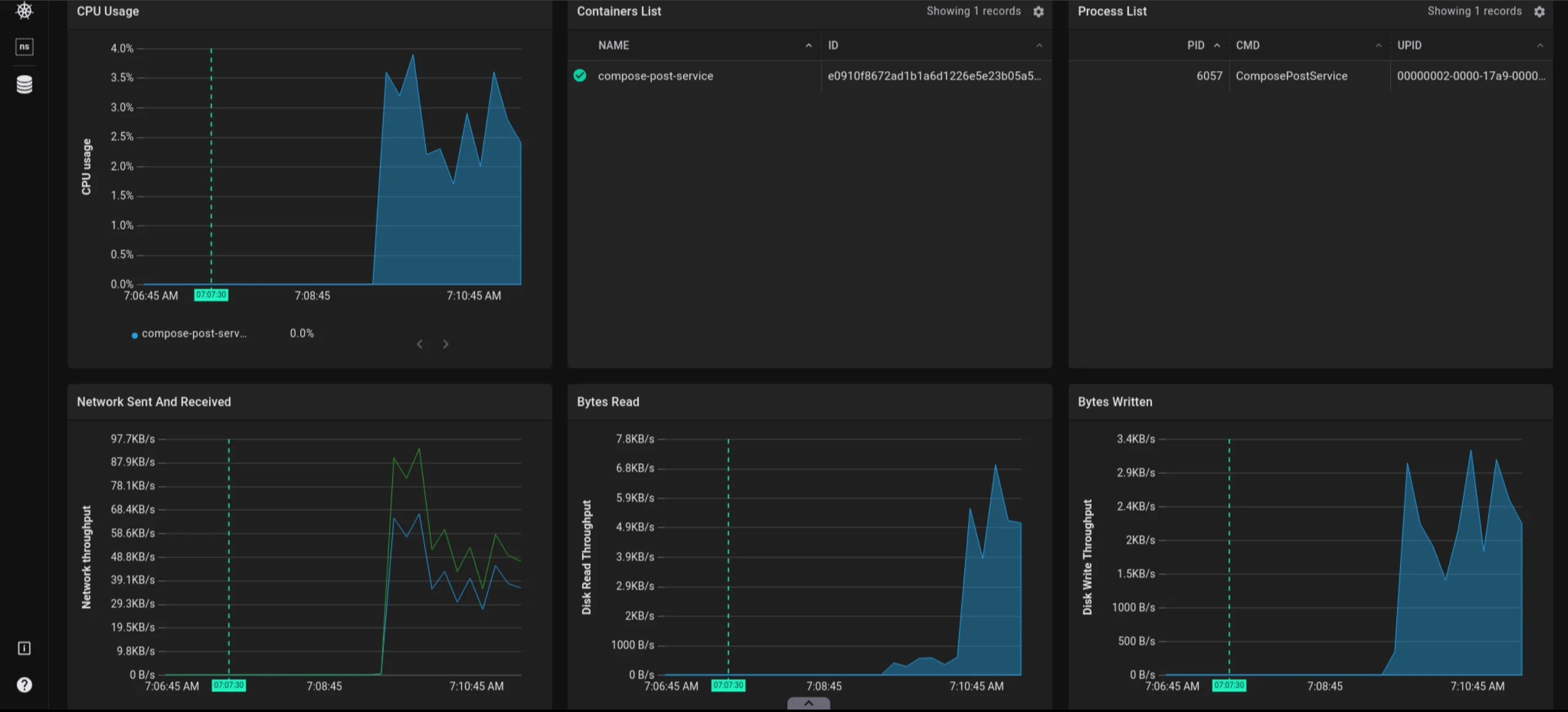
Pixie observability dashboard showing CPU usage, network throughput, and disk I/O for compose-post-service with zero application instrumentation

How it was built

The deployment ran in three stages.

1. We started with local Docker Compose: git clone --recursive, then docker-compose up -d from the socialNetwork directory, MongoDB seeded with synthetic user and post activity, wrk2 built from source, and load driven through Lua scripts. The frontend came up on port 8080 and Jaeger on 16686. The point of this stage was to validate the application before Kubernetes added its own failure modes on top.
2. Local k3s came next, migrating the Compose deployment onto Kubernetes with Helm v3 and the chart from the DeathStarBench repository. We deployed Pixie here first, partly to confirm the eBPF approach worked before spending anything on cloud infrastructure.
3. GKE came last: a zonal cluster in asia-south1-a on e2-standard-4 nodes, images pushed to Google Container Registry, helm install into a deathstarbench namespace, Jaeger and MongoDB running as cluster services, and wrk2 as a Kubernetes Job. On the cloud side we also had Cloud Monitoring, Cloud Logging and Cloud Trace/Profiler, which gave us a second and largely independent view of the same behaviour that Pixie was reporting.

Load generation used wrk2's exponential inter-arrival distribution (-D exp) against the compose-post endpoint. The parameters varied by configuration: 10 RPS with 12 threads and 400 connections over 60 seconds for the baseline, 50 RPS at the same thread and connection count for the three-replica run, and a longer, heavier test using a single thread with 8,000 connections over 300 seconds for the multi-node run.

What worked, what didn't

The single-node baseline was slow in a way that deserved more attention than we gave it at the time. At only 10 RPS, average latency came in at 30.27 seconds, with the distribution running 30.65s at p50, 41.29s at p75 and 49.41s at p90, and p99 approaching a full minute. Effective throughput settled near 6 requests per second against a 10 RPS target, so the system could not keep pace with a load that ought to have been trivial. CPU peaked around 21%, which rules out a compute ceiling and points the time somewhere else in the call chain. Over the same GKE run, compose-post-service logged 5,419 errors and cluster memory rose by roughly 20% under stress.

The more useful result came from the three-replica configuration. Running three replicas on one node should spread requests evenly across them. It did not. Replica 1 sat at about 11% CPU, Replica 2 at about 9% and Replica 3 at about 8%, against a cluster average near 10%. The GCP load balancer was not distributing evenly across pods co-located on a single node, and the likely explanations are session affinity, round-robin inefficiency within one pod pool, or lag in health checks and readiness probes. At this load the imbalance costs nothing, which is exactly why it is worth recording. It is a latent scaling defect that only becomes expensive once the pods are saturated.

Spreading the work across nodes recovered most of the balance. With three nodes running one replica each under the heavy 8,000-connection test, the system reached over 100,000 RPS, with utilisation at roughly 12%, 14% and 21% across the three nodes. That is a considerable improvement on the intra-node case even though a skew towards Node 3 remained, and it suggests that GCP's ingress path treats inter-node and intra-node distribution differently. The application is not the variable here.

One smaller observation is worth separating out. Jaeger consumed about 24% of its memory limit simply receiving traces at moderate request rates, and restarted twice during the run. Distributed tracing is not free, and on a small cluster the tracing infrastructure ends up competing for resources with the system it is supposed to be measuring.

What I'd do differently

• I would drive the replicas to saturation. The imbalance we measured at around 10% CPU is real but inconsequential at that load, and the experiment we did not run is the one that matters: push each configuration until the pods saturate, then check whether the intra-node skew turns into divergence in tail latency. Until then it is a curiosity visible in a dashboard rather than a demonstrated property of the system.
• I would also hold the load profile constant across configurations. Using 10 RPS for one setup, 50 RPS for another and an entirely different thread-and-connection shape for the third was reasonable while exploring each topology on its own terms, but it means the three are not strictly comparable, and CPU utilisation across them cannot be read as a clean curve. A fixed sweep over all three would have cost more cluster time and yielded a much stronger claim.
• Finally, I would chase the latency rather than simply reporting it. Thirty-second averages at 10 RPS indicate something specific, whether queueing in the RPC chain, a cache write path or connection pool exhaustion, and we had both the flamegraphs and the traces needed to localise it. We documented the symptom carefully and stopped short of the diagnosis.